BCS Level 123: MS Excel (Project 5)

Basic Computers Skill 1-2-3-S

Project 5

1. Open Excel and Set Up Your Headers

First, open a new, blank workbook in Excel. Then, enter the headers for your table.

Step	Action
1	In cell A2, type “Rent“.
2	In cell A3, type “Gas“.
3	In cell A4, type “Food“.
4	In cell B1, type “Jan“.
5	In cell C1, type “Feb“.
6	In cell D1, type “Mar“.
7	In cell E1, type “Apr“.
8	In cell F1, type “Total“.

Your worksheet should now look like this:

	A	B	C	D	E	F
1		Jan	Feb	Mar	Apr	Total
2	Rent
3	Gas
4	Food

2. Enter Your Data

Next, you will enter the expense data for each month.

Step	Action
1	Click on cell B2 and type “1000“.
2	Press Tab to move to cell C2 and type “1000“.
3	Continue this for all the “Rent” values.
4	In cell B3, type “55” for “Gas” in January.
5	Continue entering the rest of the data for “Gas” and “Food” in the correct cells.

Your data should now be filled in:

	A	B	C	D	E	F
1		Jan	Feb	Mar	Apr	Total
2	Rent	1000	1000	1000	1000
3	Gas	55	66	44	45
4	Food	220	300	250	290

3. Calculate the Totals with the SUM Function

Now, you can use a formula to have Excel automatically calculate the totals for you.

Step	Action
1	Click on cell F2, where the total for “Rent” will go.
2	Type `=SUM(B2:E2)` and press Enter. Excel will add up the numbers from cell B2 to E2.
3	Now, click on cell F2 again. You will see a small square in the bottom-right corner of the cell.
4	Click and drag this square down to cell F4. This will copy the formula to the other rows, automatically adjusting the cell references.

Excel will now show the calculated totals for each row.

4. Final Formatting (Optional)

To make your table look more professional, you can add some formatting.

Action	Description
Bold Headers	Select the headers in row 1 and column A. On the Home tab, click the B button to make them bold.
Add Borders	Select all the cells in your table (A1 to F4). On the Home tab, click the “Borders” dropdown and select “All Borders.”
Format as Table	For even more advanced formatting, select your data and click on Format as Table on the Home tab. This will allow you to easily apply different styles and add features like filtering.

Your final table in Excel will look just like the one we discussed, with the added benefit that the totals will automatically update if you change any of the monthly expense numbers.

Create a Chart with the Data

Create a Stacked Column Chart in Excel. This type of chart is excellent for showing how different parts contribute to a whole over time.

Here is a step-by-step guide to create that exact chart using the data.

Step 1: Set Up Your Data in Excel

First, ensure your data is organized correctly in an Excel sheet. For this chart, you will not need the “Total” column.

Open Excel and enter the data as shown below.
Make sure the expense categories are in the first column and the months are in the first row.

	A	B	C	D	E
1		Jan	Feb	Mar	Apr
2	Rent	1000	1000	1000	1000
3	Gas	55	66	44	45
4	Food	220	300	250	290

Step 2: Select the Data for the Chart

You need to tell Excel which data to include in the chart.

Step	Action
1	Click on cell A1.
2	Hold down the mouse button and drag your cursor to cell E4.
3	This will select the entire data range, including the row and column headers, which Excel will use for the chart’s legend and axis labels.

Step 3: Insert the Stacked Column Chart

Now you will insert the chart itself.

Step	Action
1	Go to the Insert tab on the Excel ribbon at the top of the screen.
2	In the “Charts” group, click on the Insert Column or Bar Chart icon.
3	A dropdown menu will appear. Under the 2-D Column section, select the second option, which is the Stacked Column chart.

Excel will immediately create the chart and place it on your worksheet.

Step 4: Customize the Chart Title

The final step is to give your chart a descriptive title, just like in the image.

Step	Action
1	Click on the default “Chart Title” text at the top of the chart.
2	A text box will appear. Delete the default text and type in “Monthly Expenses“.
3	Click anywhere outside the title box to set the new title.

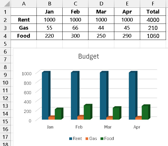
Final Result
Your chart should now look exactly like the one you uploaded. It will show the total expenses for each month, with the different colors in each column representing the breakdown of costs for rent, gas, and food.

You can click and drag the chart to move it around your worksheet or use the corner handles to resize it.

Your Project Should look like the image below