Project 6
Step-by-Step Instructions
1. Enter the Column Headings
-
Open Microsoft Excel.
-
In Row 1, enter the headings:
| Cell | Value |
|---|---|
| A1 | Items |
| B1 | Jan |
| C1 | Feb |
| D1 | Mar |
| E1 | Apr |
| F1 | May |
| G1 | Jun |
| H1 | Jul |
| I1 | Aug |
| J1 | Sep |
| K1 | Oct |
| L1 | Nov |
| M1 | Dec |
| N1 | Totals |
2. Enter the Item Names
In Column A, type the following:
| Cell | Value |
|---|---|
| A2 | rent |
| A3 | food |
| A4 | car |
| A5 | school |
| A6 | telephone |
| A7 | totals |
3. Enter the Monthly Data
Rent
Enter 1200 from B2 to M2.
Food
Enter:
| Cell | Value |
|---|---|
| B3 | 375 |
| C3 | 600 |
| D3 | 450 |
| E3 | 700 |
| F3 | 675 |
| G3 | 720 |
| H3 | 500 |
| I3 | 525 |
| J3 | 855 |
| K3 | 400 |
| L3 | 275 |
| M3 | 650 |
Car
Enter 700 from B4 to M4.
School
| Cell | Value |
|---|---|
| B5 | 35 |
| C5 | 0 |
| D5 | 250 |
| E5 | 25 |
| F5 | 25 |
| G5 | 0 |
| H5 | 0 |
| I5 | 0 |
| J5 | 250 |
| K5 | 25 |
| L5 | 10 |
| M5 | 25 |
Telephone
| Cell | Value |
|---|---|
| B6 | 150 |
| C6 | 160 |
| D6 | 140 |
| E6 | 155 |
| F6 | 140 |
| G6 | 140 |
| H6 | 150 |
| I6 | 150 |
| J6 | 150 |
| K6 | 155 |
| L6 | 155 |
| M6 | 155 |
4. Calculate Row Totals
In the Totals column (Column N) enter formulas:
| Cell | Formula |
|---|---|
| N2 | =SUM(B2:M2) |
| N3 | =SUM(B3:M3) |
| N4 | =SUM(B4:M4) |
| N5 | =SUM(B5:M5) |
| N6 | =SUM(B6:M6) |
5. Calculate Monthly Totals
In Row 7 calculate totals for each month.
| Cell | Formula |
|---|---|
| B7 | =SUM(B2:B6) |
| C7 | =SUM(C2:C6) |
| D7 | =SUM(D2:D6) |
| E7 | =SUM(E2:E6) |
| F7 | =SUM(F2:F6) |
| G7 | =SUM(G2:G6) |
| H7 | =SUM(H2:H6) |
| I7 | =SUM(I2:I6) |
| J7 | =SUM(J2:J6) |
| K7 | =SUM(K2:K6) |
| L7 | =SUM(L2:L6) |
| M7 | =SUM(M2:M6) |
6. Calculate the Grand Total
In N7 enter:
7. Create the Summary Calculations
Leave a few blank rows and enter:
| Cell | Label | Formula |
|---|---|---|
| A12 | MAX | =MAX(B7:M7) |
| A13 | MIN | =MIN(B7:M7) |
| A14 | COUNTA | =COUNTA(A2:A6) |
| A15 | AVERAGE | =AVERAGE(B7:M7) |
| A16 | SUM | =SUM(B7:M7) |
8. Format the Table
Rotate Month Headers
-
Select B1:M1.
-
Go to Home → Alignment → Orientation.
-
Choose Angle Counterclockwise.
Apply Color
-
Select B1:N1.
-
Fill with Yellow.
Borders
-
Select the whole table.
-
Click Home → Borders → All Borders.
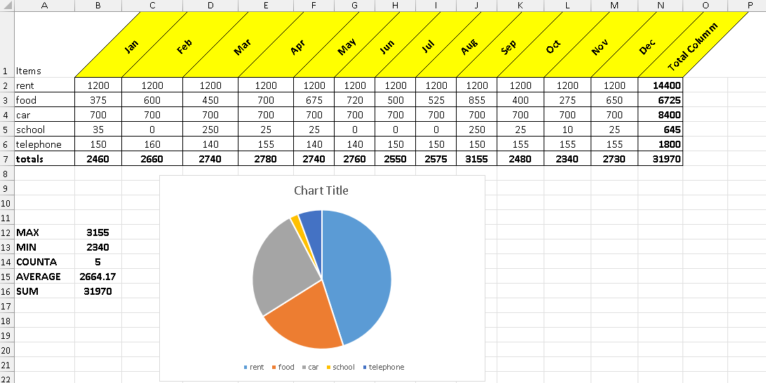
Your results should show:
-
MAX: 3155
-
MIN: 2340
-
COUNTA: 5
-
AVERAGE: 2664.17
-
SUM: 31970
Step-by-Step: Creating the Chart
1. Prepare the Data
Make sure your totals column looks like this:
| Items | Totals |
|---|---|
| rent | 14400 |
| food | 6725 |
| car | 8400 |
| school | 645 |
| telephone | 1800 |
(These values come from the Totals column of your spreadsheet.)
2. Select the Data
-
Highlight the data range containing items and totals.
-
Select:
-
Hold Ctrl and also select:
This selects both the item names and their totals.
3. Insert the Pie Chart
-
Go to the Insert tab.
-
In the Charts group, click Pie Chart.
-
Choose:
3-D Pie Chart
Excel will automatically generate a chart similar to the one in your image.
4. Resize and Position the Chart
-
Click the chart.
-
Drag the corners to make it larger.
-
Move it to an empty area of the worksheet.
5. Add Chart Title (Optional)
-
Click Chart Title.
-
Type:
6. Show the Legend
If the legend does not appear:
-
Click the chart.
-
Click the + (Chart Elements) button.
-
Check Legend.
-
Choose Right.
The legend will display:
-
rent
-
food
-
car
-
school
-
telephone
7. Improve the Chart Style (Optional)
To match the style in the image:
-
Click the chart.
-
Go to Chart Design.
-
Choose a 3-D colorful chart style.
-
You can also rotate the pie:
-
Right-click the chart.
-
Select Format Data Series.
-
Adjust Angle of First Slice.
-
8. Add Data Labels (Optional but useful)
-
Click the chart.
-
Click + (Chart Elements).
-
Select Data Labels.
-
Choose Outside End.
This will show the values or percentages on the slices.
Your results should show: